In this project, I consulted a health analytics startup on developing a predictive model for the length of hospital stay from patient data. The data were obtained from the electronic medical records of a hospital system in the form of several relational tables. The major goals of the consulting project were to
- Build an accurate predictive model for the length of patient hospital stays.
- Easily interpretable models for explanation to hospital administrative staff are preferred
- The model should allow understanding and quantification of the effect that a physician has on the length of patient hospital stays.
Why Is Knowing Patient Length of Stay (LOS) Important?
Considering that each patient day in the hospital costs approximately $1,900, and the current reimbursement system only provides a flat dollar amount per patient based on their diagnosis, without regard to the actual time spent, identifying
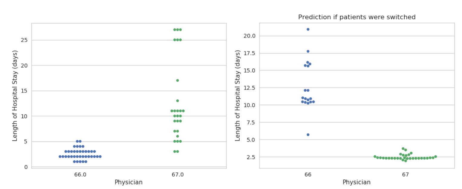
patient costs before they are incurred is the first step toward implementing cost-saving measures. One example is the effectiveness of a particular physician at resulting in a decreased length of stay for patients. In other words,
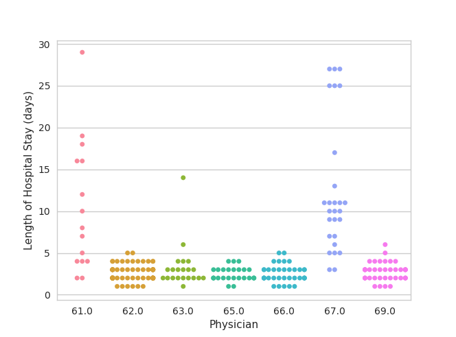
if the patient had a different doctor, would they have gotten discharged faster? For example, if we look at physicians and their patients’ lengths of hospital stays, we can clearly observe that certain physicians have more patients
with longer stays (figure 1). However, we also know that patients have widely varying conditions and the length of stay depends on the patient diagnosis in addition the the patient age and other factors that affect complexity. Taking
these factors into account can should improve the predictability of the length of stay.
Model Variable Choices
Time of prediction
Many of the features that influence the patients length of stay may evolve over the course of the visit and are correlated with the length of the visit. For example, the number of blood tests done and the number of medications given all
increase linearly with the length of the visit because patients often have daily blood tests and medication doses. However, for the model to be useful, it is important to select a time point at which the length of stay prediction is
done. I chose to predict the length of stay on day 1 of the visit in order to have the biggest opportunity of influencing the outcome. This early time point gives the administration the opportunity of optimizing physician-patient assignments.
Inclusion Criteria
The dataset were obtained from the electronic medical records of a hospital network within the region of the health analytics startup. I restricted my analysis to visits that had sufficient information to obtain the length of stay
(admission and discharge dates). I presumed that patients with very long lengths of stay, greater than a month, are there for reasons outside of the scope of their medical care and therefore excluded them from the analysis. I also
excluded patients who died during their stay. This resulted in about 40,000 remaining hospital visits. However, when grouping the patients by their type, I observed that only about 12,000 of these were inpatient visits (figure
2). Emergency room, Observation, and Nuclear Medicine visits all had very narrow LOS distribution but accounted for over half of the observations. Surprisingly, outpatient visit LOS values were very widely distributed. After discussing
this observation with the company, I learned that these patients likely came from outpatient facilities, such as nursing homes or rehab centers, which are not of interest in this analysis.
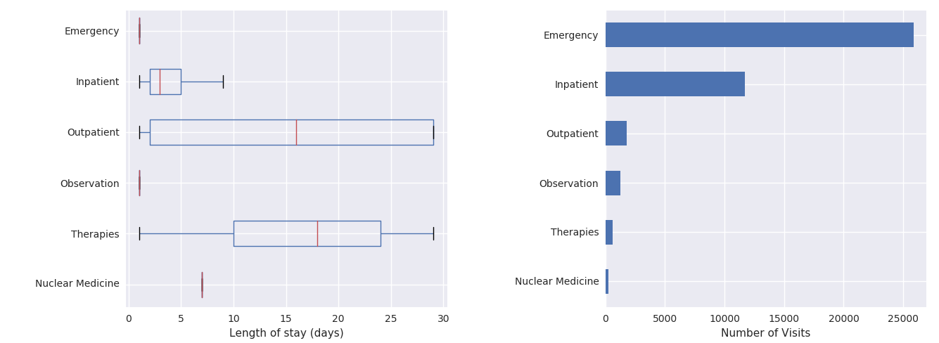
I proceeded with building a model for exclusively inpatient visits. Note that the boxplots do not show the outliers, which extend all the way out to 30 days, given the long-tailed distribution of hospital stay lengths.
Features & Model
A few preparatory steps were taken to re-package the available information into format amenable for modeling.
- A table with detailed medication data was used to count the number of medication order types each visit had within the first day. The number of different types of medications would indicated a more complex patient.
- Physician was taken as the first assigned attending physician for that patient visit.
- Patient Age was constructed from patient birth date and admission date.
- Patient Age was constructed from patient birth date and admission date.
All other available categorical variables were used, including diagnosis, facility, department, whether or not the visit is a readmission, where the patient is admitted from etc. Each of these categorical variables were 1-hot-encoded. - All sparse categories with fewer than 50 observations/category were lumped into a single group. Physicians with fewer than 10 patients were also lumped into a single group.
Treatment of Patient Diagnosis
Initially, I built a model using the diagnosis as a categorical predictor of the LOS. There were approximately 200 different diagnoses with a substantial number of observations in the data set. There was also information about the
national average LOS that corresponds to each diagnosis category. This national average LOS is used as one of the factors for determining insurance payments to the hospital. I found that models that used the mean national LOS had
a higher prediction accuracy than those that include individual diagnosis categories, and therefore used this predictor in place of the diagnosis category. Only about 75% of the patient visits had this value available, which slightly
reduced the number of visits in the model.
Baseline Model
As a baseline prediction model, I performed a regression of the observed LOS on the national average LOS for the diagnosis category. This is the predictor which is currently used by most hospital systems and is a reasonable baseline
performance metric.
Regularized Ridge Regression Model
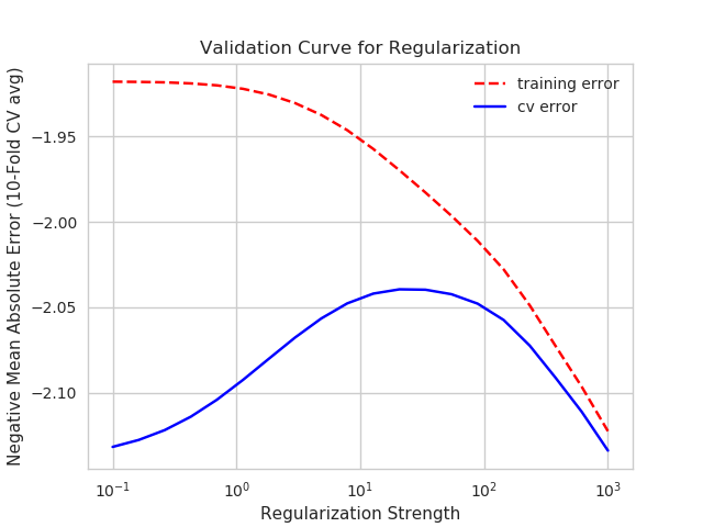
As an initial model, I performed a regularized multivariate linear regression of the LOS on all of the features, including the national mean LOS for the diagnosis. I did this using the Ridge regression from the scikit-learn Python
package. I split the data into 80% training/validation and 20% testing. I performed 10-fold cross-validation using an 80/20 training/validation split. This procedure randomly shuffles the training/validation set 10 times and splits
the set 80/20 for each shuffling instance. Learning curves showed that the model training and validation performance were very close after training on 5000 visits. The regularization strength was optimized based on the training/validation
set and gave a minor improvement (figure 4) because the training/validation errors were already very close.